
Interpretation of fMRI results
Statistical parametric maps, test hypotheses
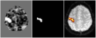
As a result of the voxel-by-voxel detection method, we obtain the so-called statistical parametric map (SPM), respectively nonparametric for nonparametric statistics. Therefore, this procedure of statistical analysis is referred to as statistical parametric (or non-parametric) mapping. The obtained statistical map contains at each point the value of the statistics coming from the respective distribution, eg the t-values of the Student's distribution. However, such a map is disadvantageous for orientation and evaluation. We, therefore, perform its thresholding, which means that for each point we have to decide on the significance or insignificance of the statistical value at this point. To do this, we set the so-called null and alternative hypothesis and the level of significance at which we perform a test deciding on the acceptance or rejection of the null hypothesis. As a null hypothesis, we determine, for example, that the average value of the signal during stimulation does not differ from the average value of the signal at rest. An alternative hypothesis then says, for example, that the value during stimulation is greater than at rest. The level of significance is then the probability with which we still admit that we can reject the null hypothesis, when in fact it is true. According to it, we check the statistical error of type I, and usually p = 0.05 is chosen for routine tests. However, such a level of significance is only suitable for fMRI in some cases, as will be discussed in the following subchapters. In the following pictures we see the original statistical map, the result after its thresholding, and finally the translation over a T2 * -weighted image of the brain.
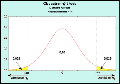
The value that determines the threshold (the statistic at a given point must exceed it in order to keep it significant) is obtained by using the appropriate probability distribution and the chosen level of significance. This actually gives us the percentage of the area under the distribution curve. According to the question asked, or the choice of null and alternative hypotheses, we distinguish between the so-called one-sided and two-sided test. In the case of a one-sided test, we consider as possible alternative cases only those when the value found is significantly higher, or significantly smaller (only one assessed option) than the considered mean value of the investigated distribution of measured data. Then we look for a threshold value only at one end of the distribution. Conversely, in the two-sided test, we ask whether the compared value is sufficiently far from the mean value (ie larger or smaller, we examine both states). Then we have to divide the level of significance, ie the area under the curve, evenly at both ends of the curve - we check both directions of difference from the mean value. In this case (also indicated in the following figure), the threshold found will be greater than in the case of a one-sided test.
Correction for multiple tests
If the voxel-by-voxel analysis is used independently and simultaneously, we test the hypothesis for many tests (we perform one test for each voxel in the brain). If we use common levels of significance (eg 0.05) in fMRI, then the resulting error valid for the whole brain will be n-fold greater (n is the number of voxels tested in the brain). For this reason, it is necessary to set a significantly stricter threshold (lower level of significance) in the fMRI, for which different corrections are used for multiple testing, eg Bonferroni corrections. We consider the thresholded statistical map to be the final map of detected activations and we will then use this to evaluate the result of the experiment.
As an uncorrected level of significance, a value of 0.001 (or 0.0001) is often used, which is used when examining predefined areas of interest, or in the survey of the whole brain in terms of the distribution of the massiveness of activations and the number of artifacts or noise.
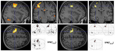
Two methods are currently used for correction. This is the so-called FWE (family-wise error) correction, in which we check the probability of a false-positive result in the whole set of tested voxels and the so-called FDR (false discovery rate) correction, in which we check the relative amount of false-positive results. Each of these correction methods then offers several possible implementations/mechanisms for calculating the decision level of significance actually used. We will only briefly mention, for example, that FWE can be implemented using Bonferroni correction (we consider truly independent tests, the resulting level of probability is obtained by dividing by the number of tests - ie tested voxels) or using the so-called "random field theory" (RFT = Random Fields Theory). This measures the degree of independence of voxels in the brain and only the number of truly independent voxels, so-called ressels) is used for correction. In the following figure, we see on the left the use of an uncorrected threshold p <0.001 and a corrected threshold using FWE for p <0.05.
Interpretation of activation maps and other results
After obtaining the activation map, a step begins in which it is necessary to perform the interpretation of the results, especially the neuroanatomical interpretation. It is an assessment of the localization of individual activated areas with respect to the functional anatomy of the brain, as well as a comparison of statistical values between individual areas and also, for example, the determination of certain time sequences during hemodynamic responses in these areas. From this information it is then possible to compile an overall model of functional activation (ie the connection between the gradual involvement of individual areas in the solution of the response to stimulation), eg using models of functional connectivity.
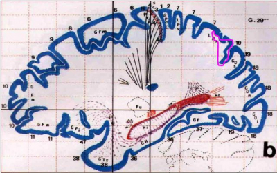
The basic step of interpretation is usually the localization of functional areas. This can be done by translating the activation map over detailed anatomical images (which requires their capture and mutual registration with functional data), when the description requires a good orientation in human brain anatomy, or by comparing the site with a brain atlas (which requires spatial transformation into a stereotactic space identical to the atlas). In practice, both methods are combined, only for the output with the preservation of the original anatomical proportions, the localization must be based only on the underlying structural images. The following figure shows the boundary of the active region (continuous cluster of voxels) transferred to the Talairach atlas.
A special case of transformation is the use of representation in cortical flat maps instead of just normalizing to the average brain template. The advantage of such an approach is the display of the results of the entire hemisphere on a single 2D image. The principle can be imagined in such a way that each hemisphere is inflated to the extent that all cortical threads are expanded and the obtained surface is then presented by decomposition into a single plane in a 2D image. An example of flat cortical maps can be seen in the following figure.
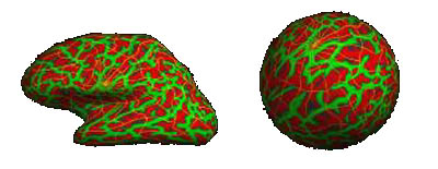
The comparison of activations in terms of the extent of the activated area and the size of the statistical values depends on the statistics used, the thresholds, and the corresponding corrections, and it should be borne in mind that a great deal of freedom is left to neuroscientists. Above all, the choice of the right threshold and the use of additional corrections for multiple testing is a step for which it is not possible to create a clear rule and in the evaluation, it is necessary to use personal experience and a certain "expert" view of a specific issue. The magnitude of the statistical values in the individual voxels is sometimes interpreted as the force of activation, which is not entirely accurate. It should be noted that when using a regression model and then estimating the regression parameters, their magnitude (also referred to as the effect strength) can be affected by the magnitude of the amplitude change of the monitored signal and the timing of the model and measured waveform. This ambiguity cannot be affected directly by test statistics and we must focus on it only when evaluating the result and subsequent verification of the statistical surveys performed and the initial assumptions used.
Finally, we mention that the interpretation is not always based on an activation map based on a statistical comparison of the BOLD effect with the course of the experiment. Another option is to display the dependence of the detected effect on another parameter, eg on the difficulty of certain stimuli compared to others, or the dependence on the order and time of presentation of individual stimuli. We can thus monitor, for example, a certain "accumulation" of the effect depending on an additional parameter, ie in general localities with a certain dependence of activation changes.


