Preprocessing of fMRI data
Principle of analysis, artifacts in data
If we successfully perform an fMRI experiment, we obtain a set of MR images as its output. If we neglect the localization images used to set the position and range of the scan, we get at least a set of images measured during a functional experiment. However, if we perform several experiments or several repetitions of the same experiment during one measurement, we also obtain several sets of functional images. These sets of function images contain the information needed to detect activation and are thus the only really necessary output from the measurements performed. In practice, however, we measure other types of images in the examined person. In particular, these are high-resolution structural anatomical images that are used as a basis for locating activated areas. Furthermore, it can be, for example, images of MR angiography used for localization of large veins (in the veins we can often observe artificial activation).
As already mentioned, the acquisition of one volume of the brain is called a scan. In one experiment, we collect a large number of scans (in the order of several tens to hundreds) that capture the state of the brain over time. We take into account the elementary volumes of the scanned space - voxels. Activation is detected statistically, separately for each voxel, based on a comparison of the time course of the signal with the course of stimulation during the experiment. This method of independently evaluating the signal in individual voxels is called voxel-by-voxel analysis. There are also methods for detection that do not require knowledge of the course of the experiment, such as principal component analysis (PCA) or independent component analysis (ICA), but they are used in a very minority. Above all, they have a problem with the neurophysiological interpretation of the result. Due to the ease of implementation and interpretation, statistical voxel-by-voxel methods are mostly used and only these will be discussed further.
As already mentioned, the analysis is based on the principle of comparing the reference and active (belonging to the moment of stimulation) state of the signal, respectively. To compare the similarity of the signal waveform with the experimental paradigm. The problems that appear in the analysis of fMRI data are mainly a small signal change (resulting in a statistical error of type II, ie false-negative results) and a large number of simultaneously examined voxels (statistical error of type I, ie false-positive results). Unlike other functional imaging methods, fMRI is extremely sensitive to head movement, which is also one of the most significant artifacts. Other artifacts result from the use of fast imaging methods (eg EPI). These are mainly ghosts, reduced sensitivity, or loss of signal around areas with a large change in magnetic susceptibility. To suppress artifacts, operations, collectively referred to as preprocessing, are performed during the analysis of functional data, which seeks to prepare the data as best as possible for statistical analysis and self-detection of activation.
Motion correction
One of the most significant artifacts in fMRI is movement. Above all, it is the movement of the head itself, but in general, most body movements are transmitted to some extent to the head. In addition, the brain itself "pulses" due to heart activity. We try to prevent the movement of the head by instructing (and motivating) the examined person and a certain form of fixation. Since no form of prevention is ideal and sometimes we intentionally limit its scope (and effectiveness), we try to further reduce the movements of the head when processing the measured data. The first scan in the functional data set is taken as a reference. For other scans, the parameters of displacements and rotations in space are then searched so that successive scans overlap as best as possible.
Correction of acquisition times
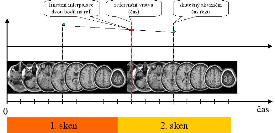
When comparing the measured data with the expected course, we assume that we captured the state of the brain in a single very short time, while the actual acquisition usually takes 2 to 4 s. In certain types of experiments and detection methods, we can afford to neglect this assumption. Conversely, some methods with rapid stimulus and inference timing comparing the time sequence of the hemodynamic response are sensitive to meeting this assumption. Thus, as a further possible pre-processing step, a method for correcting the scanning times of the individual slices is used, which tries to correct the time shifts between the individual layers by interpolating the time course. The figure shows the linear interpolation of two points in time with respect to the reference moment, which is only to show the most basic principle of the method.
Spatial normalization
The next step, which we encounter mainly in the research use of fMRI, is the transformation of images into standard stereotactic space (in fMRI called spatial normalization). This step is important for easy comparison of individual results with each other or with anatomical atlases. It allows orientation and comparison by coordinates and is therefore essential for group statistics. The essence is the transformation of images of the individual brain to the reference brain (template), which is located in a certain coordinate system, with the most commonly used Talairach coordinate system. It is possible to use not only affine linear transformations (displacements, rotations, scaling, skew) but also nonlinear deformations because we want the maximum agreement of different individual brains with a defined template. This step is debatable in the clinical use of fMRI.
Spatial smoothing
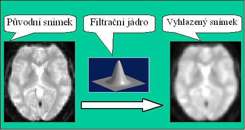
Possible operations when processing fMRI data also include spatial smoothing. It is filtering of high spatial frequencies, which tries to suppress noise in the data. As already mentioned, the signal-to-noise ratio is unsatisfactory in functional magnetic resonance imaging and we try to increase it. In addition to spatial filtering, time filtering is also used for this purpose, which will be discussed below. For spatial filtering, the Gaussian filter defined by the spatial frequency limit or parameter FWHM (full width at half maximum) is most often used. The use of spatial smoothing in fMRI has both positives and negatives, so it must be approached with caution. Some methodological methods for processing fMRI data (and the software packages based on these) completely reject it, while others require it, but most of the time it depends on the use and settings of the specific user.
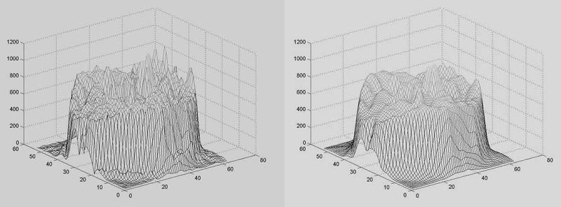
The following figure shows an example of smoothing real data. One section using a 3D graph is shown, where the z-axis represents the intensity of the image. On the left you can see the original section (after motion correction and spatial normalization), on the right you can see the same section after spatial smoothing (this was done on the entire volume, ie in 3D).

Intensity normalization
The last step, which takes place in the image (or also spatial) domain, is the global normalization of intensity. The global intensity of the BOLD signal (ie the brightness of the images) may fluctuate between acquisitions. This also affects the ability to detect activation, as the time course of the signal in a particular voxel varies according to the course of global intensity. The solution is to remove this component from the time courses in the individual voxels by normalizing the global intensity in each scan to a predetermined value. Sometimes it is necessary to omit this step in a targeted manner (eg when correlating global intensity with the course of experimental stimulation). Often, at least intensity normalization called "Grand Mean Scaling" is often used, where we calculate the average signal intensity for the whole experiment and then adjust it to a preset value. This will ensure at least comparable signal levels between individual experiments and individuals.
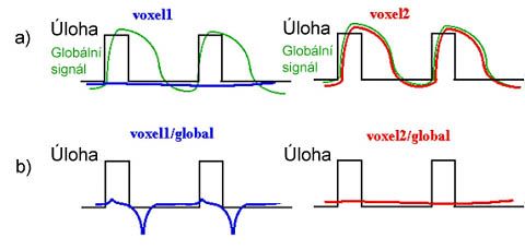
In the picture, we can see two cases of signal influence after global normalization. In the first case, the voxel shows no signal change, in the second case, the intensity in the voxel correlates significantly with the global intensity. a) indicates the original waveforms of the signal. b) indicates the result after the normalization of the global intensity. In addition to the already mentioned suppression of the correlating signal, a false negative correlation can also be induced and thus a false hypoactivation.
Time course filtering
The adjustment made only on the time course of the BOLD signal, independently in each voxel (time series belonging to the given voxel), is time filtering. We can use low and high-frequency filtering. The first one removes the slow fluctuation of the signal (it shows, for example, heart activity and respiration), the second high-frequency noise.


