
Statistical analysis
Introduction, an overview of methods
The vast majority of practically used methods for detecting activation are based on one-dimensional statistics. Methods such as principal component analysis, etc. can also be used for detection, but these cannot give us information about how the brain works or allow us to ask specific questions. Therefore, they are hardly used.
Most voxel-by-voxel methods of one-dimensional statistics require the creation of a model describing the expected course of the hemodynamic response based on the knowledge of experimental stimulation. A certain intermediate step is then deconvolution, which requires only knowledge of the beginnings of recurring events. We will now give a brief overview of one-dimensional methods and then some of them will be explained in more detail
- correlation
- t-tests
- ANOVA
- ANCOVA
- linear regression
- multiple regression
- F-tests
- etc ...
All the above methods can be implemented as special cases of the general linear model (GLM). These are the so-called parametric methods, where we assume a certain behavior of the measured data, such as the normal distribution of residues. Especially when this is not the case, non-parametric methods can also be used.
t-tests
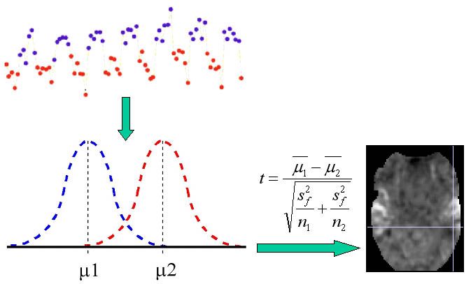
The simplest approach (and also the most susceptible to various artifacts and sensitive to well-obtained noiseless data) is a simple difference between the average value of the signal obtained during activity and the average value of the signal obtained during rest. We are able to obtain slightly better results by using a comparison of these averages by the Student's t-test, where the difference in the averages is additionally "weighted" by the standard deviation. We already take into account the variability of the data, thus avoiding some false positive detections.
Correlation and regression
The next step is higher by methods that assume a certain shape of the measured signal (we model the hemodynamic response according to the knowledge of the course of experimental stimulation). The use of correlation and regression analysis is offered here.
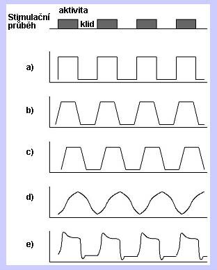
In the previous figure, we can see the course of the simulation function (simple block design) and several possible model courses. The base (a) is the periodic rectangular waveform derived from the pacing waveform. Furthermore, we can consider (b) gradual rise and fall of the measured signal, (c) certain inertia, etc. The response can also be modeled using functions (d) such as sin, cos, etc. The most perfect way in terms of mimicking real physiology is (e) convolution of the experimental course with hemodynamic function. In the next figure, we can see the indicated principle of simple linear regression, where the measured data are modeled as the sum of the constant term, the multiple of the model function, and the vector of residuals (residual variability in the data).
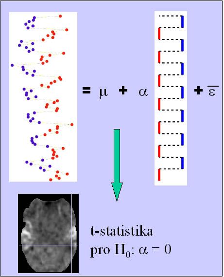
By regression analysis, we obtain a relatively flexible tool, where we try to explain the behavior of variability in the data using individual regressors (models of possible or expected response to certain types of stimuli) and then test their significance.
General linear model
A certain generalization and encapsulation of the above methods is the use of the General Linear Model (GLM). This is actually a generalization of linear regression analysis. However, depending on the method of model construction and subsequent testing and interpretation of regression coefficients, we obtain, for example, t-test or ANOVA. The basic concept is shown in the following figure.
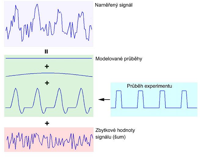
The matrix notation of a general linear model and its graphical representation can then be seen in the next figure.
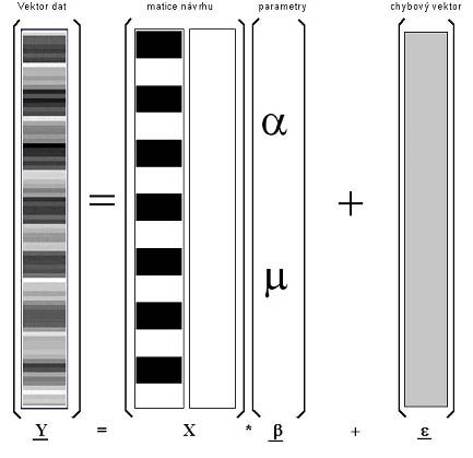
The resulting statistical picture (so-called statistical parametric map) is obtained by estimating the model parameters and calculating the relevant test statistics. To estimate the "beta" parameters of the general linear model, we use the equation from the following figure.

To calculate the test statistics, it is possible to use, for example, the equation from the following figure in the case of a requirement for t-statistics (F-statistics, z-statistics, etc. are also possible according to the method of use and interpretation).
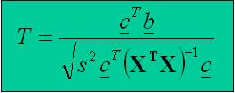
The vector c is the so-called vector of contrast weights. Using it, we determine a linear combination of estimated parameters that we will test, ie the so-called null hypothesis.


